Creating a Chart or Graph by using the Chart Wizard in MS Excel Spreadsheet
The following are the steps for creating a chart using the Chart Wizard in a Microsoft Excel Spreadsheet Software:
(1) Specify the Range
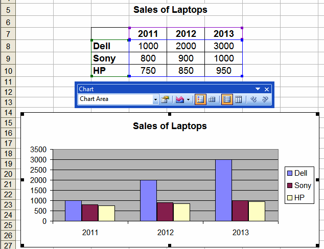
Before starting the Chart Wizard, the data to be displayed in a chart is usually selected. While selecting the data, the categories and data series names can also be selected. In the following figure, selection also includes data series and categories names. Spreadsheet ignores the corner cell because it is neither a data series name nor a chart category.
(2) Step 1 of Chart Wizard: Specify Chart Type
After selecting the data, click on Chart Wizard icon. The Step 1 of the Chart Wizard dialog box will be displayed. In this step the Chart Type is specified. The Chart Wizard provides a selection of many chart types. In addition to these, several custom chart types are also provided. A user can also specify a user-defined chart type. As a standard chart type is selected, its sub-types are displayed. Click on a sub-type to select it.
An important feature of Step 1 is the large button Press and Hold to View Sample. It is used to view the chart. Press this button. While the button is pressed, the chart is displayed based upon the series already selected. Click Next to proceed further steps.
(3) Step 2 of Chart Wizard: Specify Chart Source Data
In this step data range option, whether the chart is to be plotted in Rows or Columns and series are specified. If data has already been specified, it is shown in Data range box. To specify or change data range:
- Click in the Data range icon. The dialog will be minimized.
- Select the data from the worksheet to select the data.
- After selecting the data range, click the collapse icon to display the entire dialog box again.
To add or remove series, click on the Series tab:
- Click on Add button to add a new series.
- Specify a name and value for the new series in their respective boxes.
- Specify Category Label and click Next.
(4) Step 3 of Chart Wizard: Specify Chart Options
The Chart Options dialog contains various tabs for specifying Titles, Axes, Gridlines, Legend, Data Label and Data Tables.
- In the Titles tab type title for the chart in the Chart Title text box and hit Tab key. After a few seconds, the titles will appear in the preview window.
- In the Category (X) axis box type text for category X.
- Similarly click on each tab of the dialog and enter suitable values
- Click on Next to proceed further step.
(5) Step 4: Specify Chart Location
In Step 4, specify the location of the chart. The chart can be either within the worksheet as an object or it can be in its own sheet as a new sheet. Specify appropriate location for the chart and click Finish.
Now Click on Finish to display the chart or graph according to data or values.


